← Photo Paper Profiler  ·  IT

Photo Paper Profiler

User manual · iPhone app

Version 4.0.2 · November 2026

© 2026 adesortis · All rights reserved · www.photo-paper-profiler.com

1. Introduction

Photo Paper Profiler calculates the paper grade, the exposure time and the lens aperture for black-and-white darkroom printing, starting from light-meter readings taken on the projected negative instead of test strips. You tell the program which grey level (Zone System) you want in a few areas of the negative; the program finds the combination of grade, time and aperture that best satisfies all of them, using the profile of the paper.

The app works completely offline, has no accounts and does not collect any data. It runs on iPhone; the optional Bluetooth lightmeter connects to it with Bluetooth LE.

What you need

• an iPhone;
• a darkroom lightmeter that gives its reading as EV200 (ASA 200): the Gossen Luna with the darkroom accessory, the Gossen Vario, the Bluetooth lightmeter described in chapter 6, or your own instrument, defined in My lightmeter;
• the profile of your paper: the app includes Ilford MGFB, Ilford MGRC and Bergger PR, each in the original version and in a recalibrated one; for any other paper you can create the profile yourself (chapter 8).

Part A of this manual explains how to use the app, screen by screen; Part B describes the method behind it. This manual describes version 4.0.2. All the buttons and labels of the app are in English, and this manual uses them as they appear on the screen.

2. Quick start

A complete example, with the screens of the app.

1. At the top of the main screen choose the Paper and the Lightmeter.
2. Set Reading Ap., the lens aperture at which you read the negative (you can read at full aperture), and H head, the distance in centimetres between the lens and the paper.
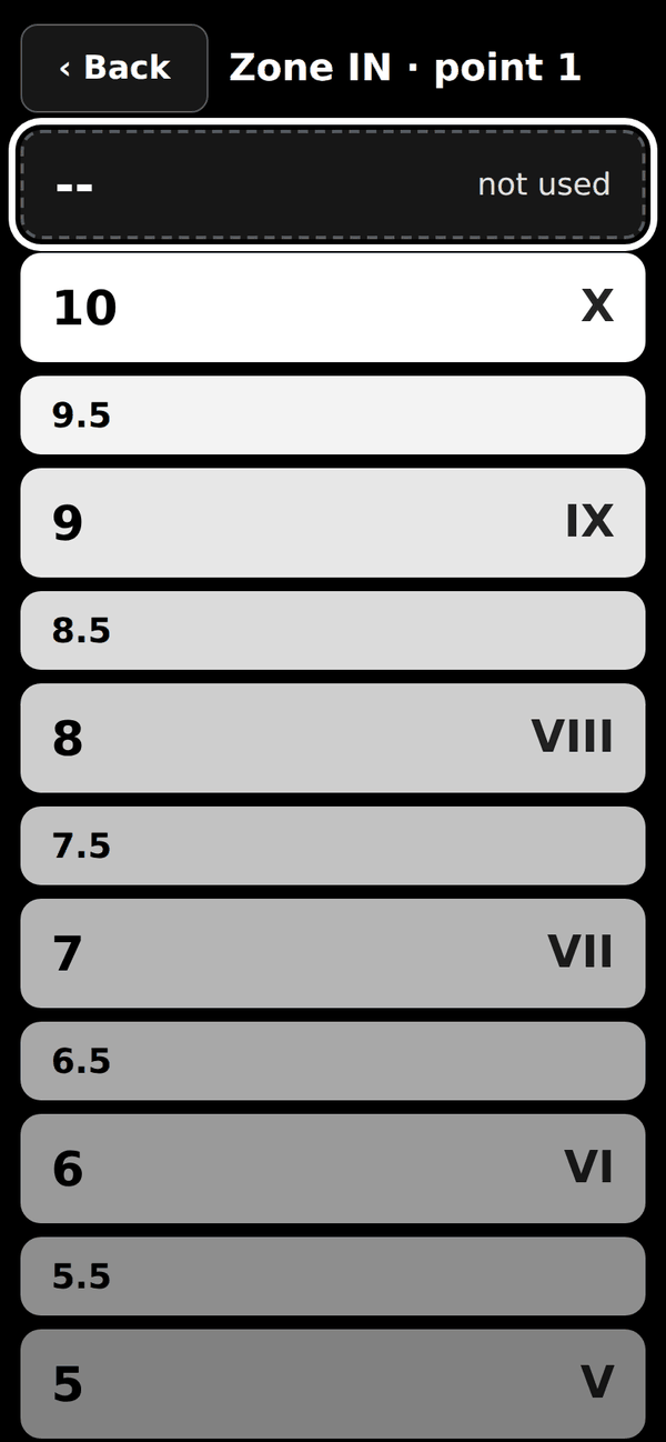
3. Read the light with your lightmeter on the areas of the negative whose grey level you want to control, typically highlights and shadows. For each area choose the reading in EV200 (at ASA 200, in 1/4-EV steps) and, in Zone IN, the grey level you want (Zone System: 0 black … X white). Tap Zone IN to open the list of the zones, each with a small square showing its grey. If the reading was taken away from the axis of the lens, type the distance in Ecc.
4. Read the result: Grade, Time (s) and Printing Ap. Next to every point, Zone OUT shows the grey level you will actually obtain; Error summarises how far the result is from what you asked for.
5. Set the grade on your enlarger and the aperture on the lens, then press Timer: a signal sounds at the start, every second during the last 3 seconds and at the end.
6. Press Save to keep the session: it appears in Saved sessions.

Grade, Time and Printing Ap. appear as soon as at least one point has both EV200 and Zone IN. To let the program choose the grade, use two or more points with Zone IN (typically highlights and shadows).

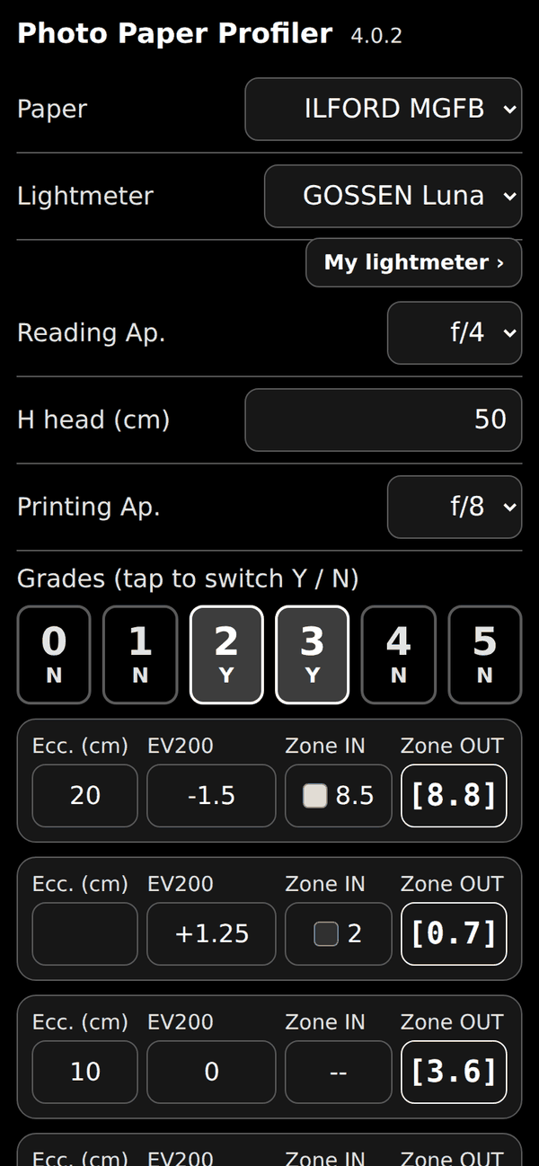
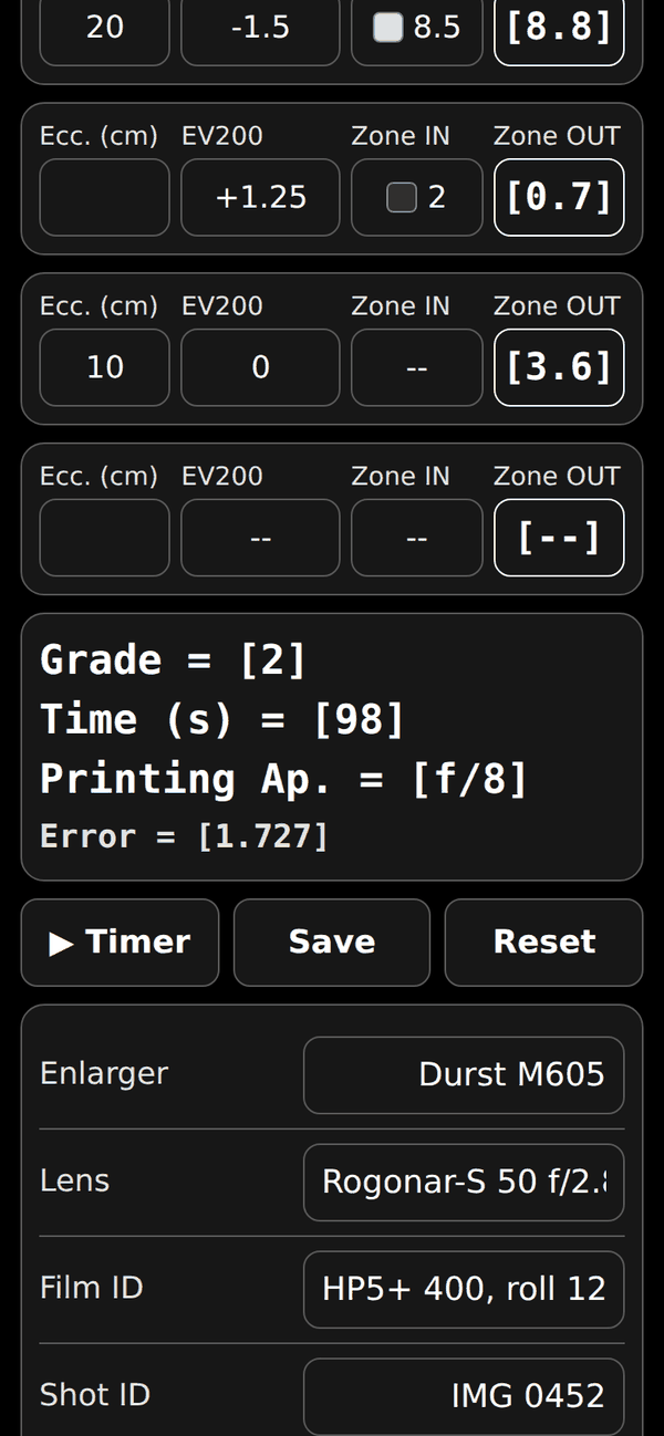
The example in the figures

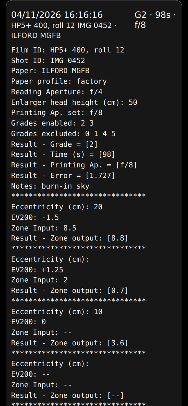
Paper Ilford MGFB; readings taken at f/4; head at 50 cm; printing at f/8 (Printing Ap.). Grades 0, 1, 4 and 5 are switched off (tap a grade to switch Y/N), so the program chooses between grades 2 and 3. Three points: (1) Ecc. 20 cm, EV200 −1.5, Zone IN 8.5; (2) EV200 +1.25, Zone IN 2; (3) Ecc. 10 cm, EV200 0, Zone IN left empty. The program proposes grade 2, 98 seconds at f/8. The obtainable grey levels are 8.8 and 0.7 for the first two points (8.5 and 2 were requested; error 1.727) and 3.6 for the third, which was not forced: for a point without Zone IN the program only tells you the grey you will obtain.

3. The main screen

3.1 Paper, lightmeter and geometry

Paper

Select the paper from the list-box. The papers marked (recal.) use curves recalculated from the author's measurements; the others are the original curves of the website. You can add your own paper profiles with Paper profiles (see below). To share a new profile with other users, export it and send the file to support@photo-paper-profiler.com.

Lightmeter

Select the lightmeter used for the measurements. If yours is not in the list, press My lightmeter and define it: sesp (height of the sensor above the paper, in cm), tara (EV shift to the corrected EV200 scale) and corr (multiplier of the negative readings, for instruments that lose sensitivity at low light; 1 if linear). The program converts every reading: (reading × corr, only if negative) + tara, and then corrects for sesp. The page explains how to find the three values.

Reading Ap.

Select the lens aperture you use when reading the EV200 values with your light meter. You can use full aperture during this stage, allowing a more accurate estimate of the negative.

H head

Input the distance in centimetres between the lens and the paper.

Printing Ap.

Lens aperture you will use for printing. If not selected, the program will suggest the lens aperture in the result box.

0 1 2 3 4 5

You can deactivate one or more paper grades selecting N. A grade shown as – is not profiled for the selected paper: it is always off and the program never uses it.

3.2 The measuring points

Ecc.

Eccentricity in centimetres of the point where you are pointing the light meter. This is the distance between the point and the axis of the lens.

EV200

Select 200 ASA as the film speed scale. Take a reading of the negative area in which you want to obtain a specific grey level, then select this value from the list-box. 1/4 EV increments are considered. During the lightmeter reading, deselect the filters of the enlarger. Negative values are unavoidable in the dark areas of the negative, but they usually fall outside the declared sensitivity of most instruments and are therefore less reliable. For this reason, you can take the measurements at full lens aperture. In any case, a correction parameter can be input, as described in the following.

Zone IN

This is the grey level you desire in correspondence of this point. The numbers correspond to that of the commonly adopted Zone System. If you do not specify any value in this field, the corresponding EV200 will not be used by the program for the optimisation. In the app, tap the field to open a list with a small square showing the grey level of each zone.

Zone OUT

This is the grey level that can be actually obtained. The program perform an optimisation, in order to approximate all Zone IN values you specify. If an EV200 value is specified and the corresponding Zone IN value is not specified, the program only calculates the grey level you will obtain in correspondence to that EV200 value. This option is useful if you do not want to force a specific area in the optimisation, but you only want to check the grey level you will obtain. In some cases, especially for very low or very high EV200 values, you could decide to perform dodging or burning, because you can’t achieve the desired grey levels for all areas. Let’s discuss the burning case, firstly. To this aim, deselect the Zone IN value corresponding to the smallest EV200 value and calculate Grade, Time and Aperture. Let’s call base time the time so calculated. Then, deselect all Zone IN values, except that corresponding to the smallest EV200 value, for which you could select 8.5, or a different value,. Be careful to check whether the Grade was not changed. In this case, force the solution using the 0 1 2 3 4 5 switches, as previously described. Now you have obtained a new time, greater than the base time. The difference between new and base time is the burning time. A similar procedure can be used to calculate the dodging time.

3.3 The results

Grade (result box)

Paper gradation (from 0 to 5). This is one of the results of the optimisation.

Time (result box)

Printing time in seconds. This is one of the results of the optimisation.

Printing Ap. (result box)

Lens aperture you will use for printing. This is one of the results of the optimisation. You can force a different aperture as described in the following.

Error (result box)

Sum of the squares of the differences between desired and obtainable grey levels. This is one of the results of the optimisation.

3.4 Data of the session

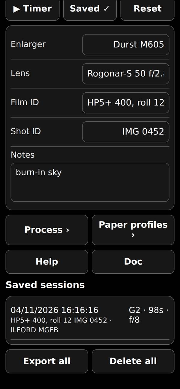
Enlarger

This is a text field, in which you can input the model of the enlarger.

Lens

This is a text field, in which you can input the model of the lens.

Film ID, Shot ID

These are two text fields, in which you can input film and shot references.

Notes

Free text field to note burning-in, masking or any other detail not covered by the other parameters. It is saved with the session and cleared by Reset.

Date/Time

Automatic field: the date and time are recorded when you save a session.

3.5 Reset, Timer and Save

Reset

Button to delete most fields, except some fields that usually you will not change during a print session.

Timer

Button to start the countdown of the calculated printing time. A signal sounds at the start, every second during the last 3 seconds and at the end. The screen stays on during the countdown.

Save

Button to save the current session: paper, parameters, results, the four points, lightmeter, enlarger, lens, film and shot references, notes, Develop, Stop and Fix times and chemicals, and the paper profile version. Date and time are recorded automatically. Sessions are stored on the phone.

3.6 Saved sessions

Saved sessions

List of the saved sessions. Tap a session to open its full report. Reload puts the session data back into the fields, Share shares the report as text and Delete removes that session.

Export all

Button to share all the saved sessions as text (for example to send them by e-mail or to save them in Notes).

Delete all

Button to delete all the saved sessions. A confirmation is requested first and the operation cannot be undone. It can be useful at the beginning of a working day, when the previous sessions have already been shared (use Export all first to keep a copy).

4. In the darkroom

In the dark room

Instructions for iPhone To avoid damage to the paper, due to the light of the iPhone screen, go to Settings - Accessibility - Display & Text Size - Colour Filters and switch on. Then select Colour Tint, slide Intensity fully to the right and Hue fully to the left. To easily select this setting, go to Settings - Accessibility - Accessibility Shortcut and select Colour Filters.
Instructions for Android Go to Settings - Accessibility - Visibility enhancements - Colour lens and switch on. Then fully slide Opacity to the right and select Red. If maximum opacity is less than 100% reduce the screen light.

The Android instructions are useful if you use the old version of the website: the Android version of the app has not been made yet.

The lightmeter too. While the USB-C cable is connected, the charging LED of the Bluetooth lightmeter is lit: it is a light that can fog the paper. Cover it with opaque tape, or charge the instrument outside the darkroom (see chapter 6.2).

5. Process: develop, stop and fix timers

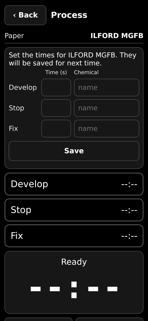
From the main screen, swipe from right to left (or tap Process) to open the Develop, Stop and Fix timers. For each stage you set the total time, in seconds, and the name of the chemical (optional): the data are saved for each paper, are requested the first time, and can be changed with Edit times.

The time of a stage includes taking the print out of the tray and letting it drain: when it expires, the next stage starts immediately. A signal sounds at the start of each stage; in the last 10 seconds a different signal sounds every second, with a rising pitch, to warn you to lift the print out of the tray and let it drain before the next bath. A final signal sounds at the end of the fixing. If you cannot hear the signals, check the volume.

Swipe from left to right to go back: the timer keeps running. When you save a print, the report also records the times and chemicals of Develop, Stop and Fix.

6. Lightmeters

6.1 My lightmeter

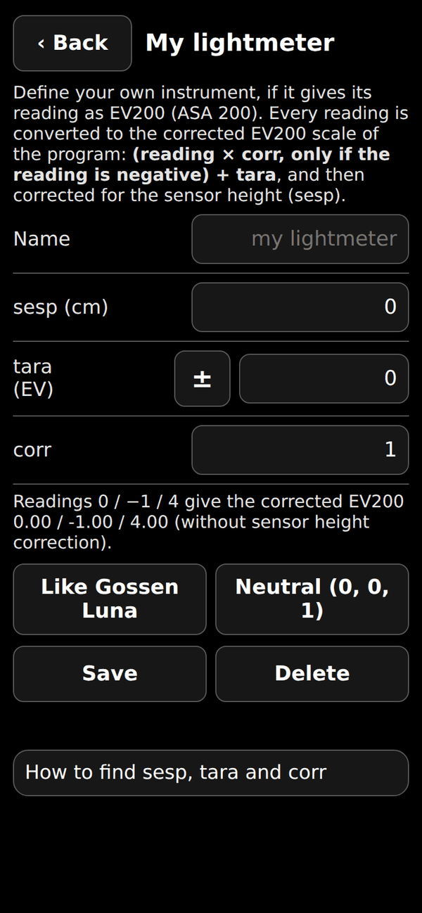
If your lightmeter is not in the list, press My lightmeter (below the Lightmeter list in the main screen) and define it: a name, sesp, tara and corr. The page shows what the three values do: for readings 0, −1 and 4 it gives the corrected EV200. Like Gossen Luna fills the fields with the values of the Gossen Luna, Neutral (0, 0, 1) leaves the readings unchanged; Save and Delete keep or remove your instrument, which then appears in the list.

How to find sesp, tara and corr

• sesp: height of the sensor above the printing plane, in cm. The program corrects the reading to the paper plane: ΔEV = 2·log₂((H − sesp)/H).
• tara: shifts your readings to the corrected EV200 scale, where EV200 = log₂(lux / 2.6) + 1 (the constant 2.6 is the one of the VEML7700 instrument). Read the same light with your lightmeter and with a reference, where your lightmeter is reliable, and take the mean of (reference EV200 − your reading). The Gossen Luna with the darkroom accessory reads 0 when the corrected EV200 is −2: tara = −2.
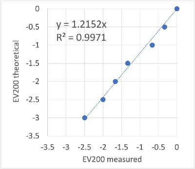
• corr: multiplies the readings that are negative on your lightmeter (before tara). If your instrument loses sensitivity at low light, change the light by one stop at a time with the lens aperture and take the slope of the true EV200 against the measured one for the negative readings (Gossen Luna: 1.2152). If it stays linear, corr = 1.

6.2 The Bluetooth lightmeter

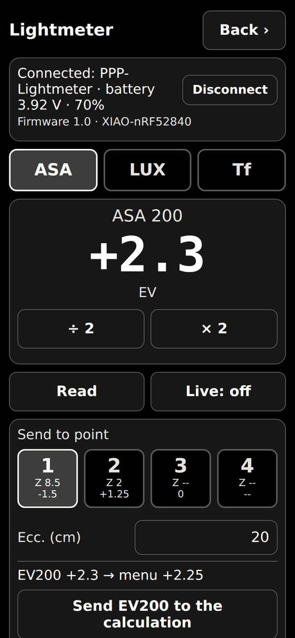
Select the lightmeter Bluetooth to unlock the lightmeter page: tap ‹ Lightmeter or swipe from left to right. Connect the instrument via Bluetooth (Connect: with the instrument switch ON, choose PPP-Lightmeter from the list; the first time iOS asks for Bluetooth permission) and press Read, or Live for continuous readings. Under the connection status the app shows the firmware version of the lightmeter (for example “Firmware 1.0 · XIAO-nRF52840”).

There are three modes, as on the instrument: ASA shows the EV at the selected ASA (÷ 2 and × 2 change the ASA), LUX shows the illuminance in lux, Tf shows the f-number to use for the selected time (÷ 2 and × 2 change the time). In Tf mode the ASA used is the one set in the ASA section. The Tf mode has nothing to do with printing the negative: it can be used when the external lightmeter connected via Bluetooth is used as an ordinary incident-light meter.

In that case, however, it would have to be calibrated with a suitable diffuser, which may be done in a future version of the program.

To use a reading in the calculation, select a point (1-4), type its eccentricity if you want, and press Send EV200 to the calculation: the EV200 (always at ASA 200, in the nearest 1/4 EV step of the menu) is written in the fields of that point and the next point is selected. If Zone IN is not yet set for that point, the Zone IN list opens right after sending, so you can choose the zone you want for the area you are measuring, and then you return to the lightmeter page; if Zone IN is already set, the page stays as it is. Simulator lets you try the page without the instrument. Swipe from right to left, or press Back, to return.

Readings and battery

In dim light a reading can take several seconds: the instrument waits as long as needed for a reliable value (up to 60 seconds). Meanwhile the screen shows …read and, after a few seconds, Reading: wait with the seconds elapsed, and sending stays disabled: the app never shows an old value as if it were new. In Live the value fades if no update arrives for 2 seconds.

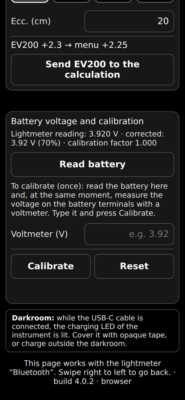
The battery voltage and charge appear next to the connection status (for example 3.87 V · 62%; the percentage comes from the discharge curve of a LiPo cell and is indicative); with the firmware 0.5 or later they are shown as soon as the connection is made. When the voltage is below 3.5 V the message Battery low: recharge the lightmeter appears.

In the section Battery voltage and calibration you can read the battery at any time and calibrate it once: read the battery in the app, measure the voltage on the battery terminals with a voltmeter at the same moment, type it in Voltmeter (V) and press Calibrate; Reset removes the calibration. Too dark to read means that the light is below the lowest level the instrument can measure.

The instrument must be switched ON to charge its battery from the USB-C port. Darkroom warning: while the cable is connected, the charging LED of the board is lit; it is a light that can fog the paper, so cover it with opaque tape or charge the instrument outside the darkroom.

7. Paper profiles

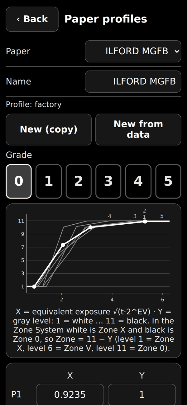
The Paper profiles button opens the calibration curves of each paper. For every grade (0-5) there are 4 points (X, Y): X is the equivalent exposure, Y the gray level: 1 = white … 11 = black. In the Zone System white is Zone X and black is Zone 0, so Zone = 11 − Y (level 1 = Zone X, level 6 = Zone V, level 11 = Zone 0). To the left of P1 and to the right of P4 the curve stays horizontal (the white of the paper and its maximum black): the chart shows these stretches too.

You can edit the curves, create a new paper with New (copy) (it starts from a copy of the selected one) or from your own measurements with New from data (see Profiling a new paper), write the development conditions in Notes, and rename or delete the paper. Factory papers cannot be deleted and, if edited, can be restored with Reset to factory. Export saves all profiles in a JSON file (paper-profiles.json) and Import loads them from a file: papers with the same id are replaced, the others are added, and Undo last import reverts the last import.

The file is saved in the format of version 4.0 (the feq of the curves are on the corrected EV200 scale); files of the previous format are converted when imported. Every saved print records the profile version used (Paper profile). To share a new profile with other users, export it and send the file to support@photo-paper-profiler.com.

8. Profiling a new paper

A paper profile tells the program how dark the paper becomes for a given amount of light. For each grade (0-5) there are 4 points (X, Y): X is the equivalent exposure feq = √(T·2^EV200), where T is the exposure time in seconds and EV200 the light on the paper in the corrected scale of the program (see below); Y is the gray level on a scale of 11 levels (1 = white … 11 = black; in the Zone System Zone = 11 − Y, so level 1 is Zone X and level 11 is Zone 0). Below P1 the curve stays at the white of the paper, above P4 at its maximum black.

The EV200 scale

The program works with a corrected scale, EV200 = log₂(lux / 2.6) + 1. Every lightmeter reading is converted to it: (reading × corr, only if negative) + tara, and then corrected for the height of the sensor above the paper (sesp). The values of the lightmeters in the list are built in; for another instrument use My lightmeter in the main screen. For example, the Gossen Luna with the darkroom accessory has tara −2: its reading 0 is EV200 −2.

Terms

A sheet is an uncut sheet of photographic paper; a sheet section is a part of a sheet used to make strips; a strip is a part of a sheet with the same exposure.

What you need

Six sheets of the paper (about 18 × 24 cm), one for each grade 0 to 5 (fewer if you profile only some grades); a negative with a uniform gray frame (for example the photograph of an evenly lit light-box taken with different apertures or times, choosing the best one); your lightmeter; a scale with exactly 11 gray levels (1 = white … 11 = black) to read the results: for example the B.I.G. Test Plate RES7 (used by the author), or a reflective chart with an 11-step gray scale such as the Image Engineering TE153 or TE83.

Two plans

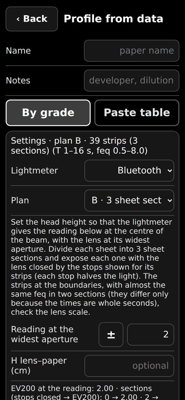
The whole profile depends on one light level, so it is better to read it where the lightmeter is reliable. Plan A: for each grade you expose one sheet; the whole sheet is one sheet section, with 40 strips all at one light level, EV200 −2: times up to about 4 minutes, and the level is read where lightmeters are less reliable; you can also read at a higher level and then close the lens by some stops (type them in the app). Plan B (recommended): you read the light once, at the widest aperture of the lens, with the lightmeter at about EV200 +2 (the app tells you which reading to aim for on your instrument); then, for each grade, you divide the sheet into 3 sheet sections, one for each reduction of the lens aperture (0, 2 and 4 stops: EV200 +2, 0 and −2), with 13 strips in each (39 per sheet).

The times are short (up to 16 s) and the level is not read where the instrument is least accurate. The strips at the boundaries (almost the same feq in two sections: they differ only because the times are whole seconds) check the lens scale. An error of 0.1 EV on the reference level changes all the final times by 7%.

1. Light

Raise or lower the enlarger head until the lightmeter gives the reading shown by the app (plan B: at the widest aperture) at the centre of the beam, and keep the head height unchanged for the whole test: in plan B only the lens aperture changes, from one sheet section to the next. The beam must cover the sheets generously. At the widest aperture the beam is less uniform: keep the strips of that sheet section near the centre.

2. Strips

On each sheet section make the strips with masks, exposing them for growing times T. Choose the range of feq to explore (we suggest from 0.5 to 8) and the number of strips (40 per sheet in plan A, 13 per sheet section in plan B): the times follow from the EV200 of each section, and are whole seconds spread regularly on a logarithmic scale between the two feq (the first ones are consecutive seconds). In plan B the steep part of the curve is exposed with times from 4 s on, in steps of 1 s, where the error of the timer weighs less.

The app (Suggest times) and the spreadsheet compute them in the same way and show the feq of every strip; you can edit the times if you need to. Develop, stop and fix as the paper maker recommends and write down the conditions (developer, dilution, time, temperature).

3. Reading

Compare each strip with the 11-level strip and write down its gray level, from 1 (white) to 11 (black); use decimals (for example 5.33) when it falls between two levels. Judge all the strips in the same way.

4. Spreadsheet

The file profiling-template.xlsx (download it from photo-paper-profiler.com/profiling-template.xlsx) has four tabs: Instructions, Plan A, Plan B and an Example with real measurements (plan A). In the tab of your plan write H (distance lens-paper in cm), sesp, tara and corr of your lightmeter and the reading (J3:J7): the tab converts it to the corrected EV200, tells you which reading to aim for, and writes the times; then write the gray level of each grade in the yellow cells. The chart shows the points: they should form a smooth S curve, so correct any typing errors.

5. In the app

In Paper profiles press New from data and type the name of the paper (and in Notes the development conditions).

The measurements can be entered in two ways.
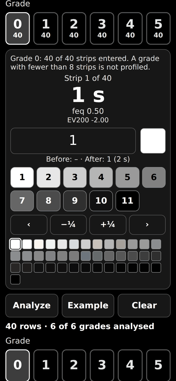
By grade (the one for the iPhone, with your prints in front of you): in Settings choose your lightmeter and the plan, and write the reading you took (the app shows the reading to aim for and, for each strip, its EV200, its sheet section and the stops to close); if you want the correction for the height of the sensor write H. The strip times follow your settings (Suggest times recalculates them, or you can type your own: in plan B one line per sheet section, “stops closed: times”).

Then choose the grade (0-5): the app shows one strip at a time, with its time and feq. Compare the print with your reference scale and type the gray level (the small square shows the gray you entered), or tap a level of the scale; ‹ › go to the previous and the next strip, −¼ +¼ adjust the value (an empty strip starts from the value of the previous one), and the small squares at the bottom show all the strips: tap one to jump to it. Leave empty a strip you did not read.

The number under each grade counts the strips entered. You can profile only some grades: a grade with fewer than 8 strips is not profiled, and for that paper its button in the main screen is always off. What you enter stays on the device until you press Clear, so you can continue later.
Paste table (handy if you already have the data in a spreadsheet): paste columns A to H of the spreadsheet (rows with data, without the header). The EV200 column is already in the corrected scale: no conversion is applied.
In both cases press Analyze. Example loads real measurements to try the procedure.

For each grade the program finds the 4 points that best follow your measurements: the chart shows your measurements (circles) and the fitted curve, and the text gives the RMS error and the largest error, in gray levels. Check the grades 0 to 5 one by one: if you are not satisfied, correct P1…P4 by hand (Automatic fit restores the calculated points). When the grades you want are good, press Save as new profile: the paper is added to the list. At least 8 measurements per grade are needed.

6. Check and share

Make a test print and compare it with what the program predicts; refine the profile if needed. To share it with other users, use Export and send the file to support@photo-paper-profiler.com, with the development conditions in Notes.

9. Introduction to the method

One of the most used methods for black and white printing in the darkroom is based on the so-called test strips. By applying this method, a gradation of the paper and an aperture of the diaphragm are chosen, after which the paper is exposed with increasing times following a sequence at regular increments, or at increments of submultiples of f/stop. Examine the strips and find the most satisfying one for the highlights. If the shadows are also rendered satisfactorily, the test is over.

On the other hand, if the shadows are rendered satisfactorily for longer times, the gradation of the paper must be increased, vice versa the gradation of the paper must be reduced. If you change gradation, you have to start over with a new test strip. After the right gradation and the best time have been found, it may be appropriate to refine the latter by repeating the strip with smaller increments of time, in order to achieve the desired result. This procedure involves a waste of time and paper consumption, although the operator's experience can lead to a significant reduction in both.

In the past, many electronic tools have been produced to automate the choice of printing parameters. Even more recently, devices based on functionality similar to those of the discontinued items have been placed on the market. These products have a significant cost and are related to the assistance and technical support of manufacturers. They usually provide the possibility for the user to introduce their own paper profiling parameters. There are no calculation tools, like this, that allow using standard darkroom light meters to obtain the same results without purchasing dedicated electronic tools.

In the procedure proposed in this document, we explore the possibility of selecting the gradation-time pair without going through the test strips. The procedure is based on the brightness levels of the various parts of the negative projected by the enlarger. A calculation tool developed for this purpose is responsible for optimizing the choice of printing parameters.

10. The measuring tool

In order to measure the various areas of a negative in a repeatable manner, it is necessary to use a darkroom light meter. In the case treated here, a Gossen Luna-Pro F was used with the accessory called LAB attachment.

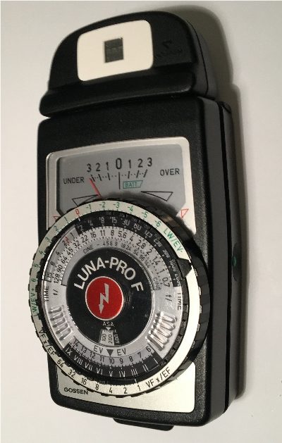
The light meter measures the light level (in lux). The graph below shows the relationship between lux and EV100 of the instrument (points) together with the analytical expression.

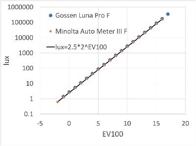
The EV scale is linear, while that in lux is logarithmic. It is important to take into account the fact that light meters measure an intensity of illumination per unit of surface. Therefore the measured EV value should not vary from instrument to instrument, as can be seen from the graph, which also shows the lux-EV relationship of the Minolta Auto Meter III F, which can be superimposed on that of the Gossen.

Ultimately, even if different exposure meters have different sensor sizes, for the simple fact that the measurement in lux (from which the EV is derived) is expressed per unit area, the result should not change by changing the reading instrument.The major limit of the instrument is related to its sensitivity, which usually corresponds to EV200 = 0. This means that, if the lens diaphragm is closed and a reading of a dark area of the negative is taken, negative EV200 values can be found, and therefore not entirely reliable because they are below the sensitivity of the instrument.

This problem can be solved in two ways. The more rigorous approach involves taking the exposure meter readings of the negative at full aperture, and then recalculating the print exposure based on the diaphragms normally used. An approximate approach is based on some simple experiments, with which a correction coefficient is calculated to take into account the measurement error below the threshold of the instrument. Let us see how to proceed to calculate the correction coefficient. We know that closing the lens diaphragm by one stop reduces the EV200 value by one unit.

This is easily verified by positioning the light meter in the center of the projected image, even without a negative, by moving the enlarger head until reading, for example EV200 = 3 at full aperture, for example at f/4. If we close at f/5.6 we will read EV200 = 2, at f/8 we will read EV200 = 1, at f/11 EV200 = 0. So we verified that the lens diaphragm correctly selects the variation of light. Now we can raise the head of the enlarger until, at f/4, we read EV200 = 0 with the light meter.

By repeating the previous steps, we can note the values of EV200 measured by the instrument, which generally do not follow the sequence that we expect: EV200 = 0, -1, -2, -3. Plotting the measured and theoretical values in a graph, we see that the points align themselves approximately on a straight line, for which it is possible to calculate the angular coefficient, which represents the desired corrective coefficient to be used in the measurements.

Another aspect to be taken into account in the light measurements on the printing surface is that of the physical dimensions of the instrument. This means that the light level is measured at a certain distance from the paper and therefore, especially if the head is low enough, an error is made, which can be taken into account knowing that the light level decreases with the square of the distance.

Finally, we can take into account the so-called cosine-correction term, representative of the fact that when the angle formed by the direction of the luminous flux that hits the instrument cell with the normal to the plane of the cell is different from 0, the quantity of measured light decreases with the cosine of the angle. Then a corrective factor can be applied to derive the light intensity that would have been measured under ideal conditions.

The above reported calibrations have been applied to the lightmeters selectable with the corresponding listbox of the app.

11. Paper profiling

The purpose of profiling a printing paper is to find a functional relationship between the amount of light to which the paper is exposed and the grey level. The amount of light depends on many factors: the negative, the height of the enlarger head, the lens diaphragm and the printing time. A variable that further increases the factors to be considered is also given by the gradation of the paper or filter. The chemicals used also affect the final result, but if you follow the manufacturer's standard guidelines their influence is less pronounced than the other factors listed above.

A sample strip with 11 gray levels (1 = white to 11 = black) was used in the procedure described here. It is immediate to find the correspondence with the Zone System which, as is known, goes from Zone 0 = black to Zone X = white. The procedure requires 6 sheets of the paper to be profiled. Each of the 6 sheets is printed with the different grades of the filter (from 0 to 5). The enlarger head must be positioned in such a way as to project a light beam that covers the printing area with a certain abundance.

It is advisable to use a negative in which the entire frame has a uniform level of gray. In the profiling, the negative and the height of the head have been selected in order to measure exactly EV200 = 0. This is Plan A, described in chapter 8 (the reading 0 of the Gossen Luna corresponds to EV200 −2 on the corrected scale of the program). For each gradation of the filter and for each printing time, a strip is obtained to be compared with the sample gray levels.

Each paper and each gradation express specific characteristics, which can be appropriately selected by the operator during the printing phase. The usefulness of this representation of the relationship between light intensity and gray level lies in the fact that it is possible to measure a limited area of a negative and obtain the EV200 exposure value. If a precise gray level is wanted to be associated with this area, it is possible to enter into the profiling curve with the gray level and obtain aperture, printing time and gradation of the paper.

12. The calculation tool

We have previously discussed how you can derive the printing time, the aperture and the gradation of the paper, once the brightness level of the negative is known, depending on the desired gray level of the final printing. This operation, however, normally does not refer to a single area of the negative, but to several areas, for each of which a specific level of grey is desired, depending on the expressive result to be obtained. In mathematical terms, the problem can be defined as an optimization problem, as we seek the gradation-time combination that best satisfies the desired result.

To speed up the procedure it is advisable to use this calculation tool. For several areas of the negative in which you intend to impose different grey levels, perform a reading with the light meter at ISO 200, eventually noting an eccentricity, i.e. the distance between the axis of the lens and the point where the measurement is made. Knowing the aperture of the diaphragm at which the light reading is made, the code finds the best time-gradation pair that respects the desired levels (expressed with the Zone System).

The obtainable result is shown next to each cell, while the overall square error provides a global indication. When a Zone value is not requested in correspondence with a value of EV200, the code simply calculates the grey level corresponding to the optimization performed, which instead is guided by the cells for which a Zone value is provided. If the printing opening calculated by the code is not convenient, it can be forced, resulting in a recalculation of the printing time. It is possible to deactivate some gradations of the filters, to force the optimization on the desired ones.

13. A worked example

To illustrate the usefulness of the code with a practical case, we start from the negative shown on the following.

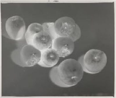
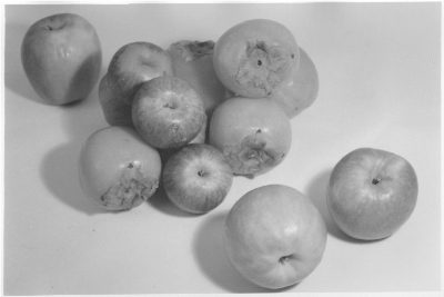
Exposure readings were taken with a Durst Neonon 105 mm 1: 5.6 lens at full aperture. Highlights reading provide EV200 = 2.67, while deep shadows provide EV200 = 4. By imposing a Zone VII for the former and a Zone I for the latter, the code calculates a grade 3, with a time of 21 sec at f/16 aperture. Ilford MGFB paper was used. Compared to the required values, the obtainable Zones are respectively 7 and 0.9, therefore very close to those in input. The result is shown below.

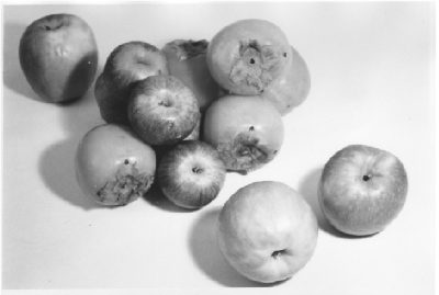
By associating Zone VIII and Zone 0 to the highlights and to the deep shadows, respectively, the code calculates a paper grade 5, with a time of 12 sec at f/16 aperture. Ilford MGFB paper was also used in this case. Compared to the required values, the obtainable Zones are respectively 7.8 and 0.7. The result is shown below.

14. Conclusions

The printing procedure most commonly used in the darkroom for black and white is based on test strips, with which, by successive approximations, the correct gradation-time coupling is found to achieve the desired expressive result. Each paper is characterized by a profile, defined as the relationship between the intensity of the light flux and the grey level. Knowing this profile, and effectively measuring the light projected by the negative on the paper, it is theoretically possible to predict the final result.

The procedure proposed here is based on the use of a fairly common instrument, namely a light meter equipped with an accessory to measure the light level of different areas of a negative. Some aspects related to the accuracy of the measurement were investigated, as it was observed from the various experiments that this accuracy plays a very important role in the possibility of actually obtaining the results expected from the calculation. Subsequently, the profiling of the paper was discussed, carrying out test strips and associating the corresponding grey levels to the various times, and to the various paper grades.

Profiling is incorporated into a calculation tool, with which we can optimize the two parameters of interest (grade and time) to obtain the smallest difference between desired and achievable grey levels. Some experiments, including an example discussed in detail in the text, have shown an acceptable accuracy of the instrument. Obviously, the achievement of the optimal result could also require subsequent steps, such as dodging and burning, as well as further refinements of the printing time, starting however from a solution not too far from the final one. Thus, a significant saving of time and material is possible.

One way to derive the burning or dodging time is described below. For simplicity, let's imagine we want to calculate the burning time. Let's suppose we have imposed some printing parameters on the highlights, but having renounced a darkening of the highest lights. From reading with the light meter on these areas, freeing all the others, imposing a VII-IX gray level and forcing the calculation to the previously determined grade and aperture, a longer time is obtained. The difference between the new time and the calculated one gives the necessary burning time. The same can be said for dodging.

In this case we will get a shorter time. The difference between these two times will tell us how much we have to dodge to lighten the areas of interest.

Contacts: support@photo-paper-profiler.com

A. Troubleshooting and questions

I enter EV200 but no result appears.

Grade, Time and Printing Ap. appear as soon as at least one point has both EV200 and Zone IN. A point with EV200 but without Zone IN is not used for the calculation: it only shows, in Zone OUT, the grey you will obtain. To let the program choose the grade, use two or more points with Zone IN.

What does Error mean?

It is the sum of the squares of the differences between the grey levels you requested and those you can obtain. The closer to 0, the closer the print will be to what you asked for.

A grade button shows “–”.

That grade is not profiled for the selected paper: it is always off and the program never uses it.

My lightmeter gives negative EV200 readings.

They are normal for the dark areas of the negative: they are unavoidable. With many instruments, however, negative values are less reliable, because they fall below the declared sensitivity. Take the readings at full lens aperture and set Reading Ap. accordingly; if your instrument loses sensitivity at low light, define its correction in My lightmeter (chapters 3.1 and 6.1).

The Lightmeter page says “Too dark to read”.

The light is below the lowest level the instrument can measure. Read at a wider aperture and set Reading Ap. accordingly.

A reading takes several seconds.

In dim light the instrument waits as long as needed for a reliable value (up to 60 seconds). Meanwhile the screen shows …read and sending is disabled: the app never shows an old value as if it were new.

The app does not find the Bluetooth lightmeter.

Switch the instrument ON, press Connect and choose PPP-Lightmeter from the list. The first time, iOS asks for the Bluetooth permission: if you refused it, allow it in the Settings of the iPhone, in the page of the app. If the message Battery low appears, recharge the instrument.

The charging LED of the instrument lights up when I connect the USB-C cable to the iPhone.

It is normal: an iPhone with USB-C supplies power and the instrument charges its battery (the switch must be ON). In the darkroom the LED is a light that can fog the paper: cover it with opaque tape or charge outside the darkroom. While the cable is connected, the voltage and the percentage shown by the app include the voltage of the charger: to judge the battery, disconnect the cable and wait about ten minutes.

How do I protect the paper from the light of the iPhone screen?

Use the colour filters of iOS (or the colour lens of Android), as described in chapter 4.

I changed phone or reinstalled the app: where are my data?

The data are stored on the phone, and deleting the app deletes them. Before changing phone or reinstalling, in Paper profiles press Export and keep the file (then Import on the new one); the saved sessions can be shared as text with Export all.

There is no sound from the timers.

Check the volume of the iPhone.

Where do I send a new paper profile?

Export it from Paper profiles and send the file to support@photo-paper-profiler.com, with the development conditions in the Notes of the profile.

Does the app send my data anywhere?

No. The app works completely offline and does not collect or transmit any data; see the privacy policy on the website.

B. Release notes

C. Licence, credits and contacts

© 2026 adesortis. All rights reserved. No source code is published. The app, the lightmeter firmware, its case files, this manual and the paper data are free to download and use, including for professional darkroom work. They may not be copied, modified, redistributed, or used for a commercial purpose (selling, paid courses or workshops, monetised content such as YouTube videos) without the author's written permission. To ask for permission for a commercial use, write to support@photo-paper-profiler.com. Full text on the website: www.photo-paper-profiler.com.

Building the lightmeter is at your own risk: it is a photographic instrument, not a safety device, and is not meant to measure anything hazardous.

Durst, Gossen, Bergger, Ilford and the other product and company names mentioned are trademarks of their respective owners; the project is not affiliated with any of them.

The iPhone version was developed with the help of Claude, an AI assistant by Anthropic (see the release notes).

Contacts: support@photo-paper-profiler.com